Exploring Mouse PDAC RNA-seq: Npy1r Knockout, QC, and Deconvolution

2026-09-06

In this blog post, we begin with a bulk RNA-seq dataset from a mouse model of pancreatic ductal adenocarcinoma (PDAC). We introduce the analytical gap by showing that genotype contrasts alone rarely explain the dominant structure in tumour transcriptomes. We then walk through a reproducible exploration pipeline, from GEO data acquisition and count QC through filtering, TMM normalisation, PCA, and mouse-aware cell-type deconvolution. The post showcases the core exploratory findings for an Npy1r knockout versus wild-type contrast and explains why they matter for interpreting stromal and immune signals in PDAC. Finally, we conclude with practical implications for differential expression design and follow-up analyses.

Introduction and Background

Pancreatic ductal adenocarcinoma is a stroma-rich malignancy in which epithelial tumour cells coexist with cancer-associated fibroblasts (CAFs), immune infiltrates, and extracellular matrix. Bulk RNA-seq of tumour tissue therefore reflects a mixture of cell states, not a pure epithelial signal. When comparing genotypes, here, Npy1r knockout (KO) versus wild-type (WT) mice in a PDAC-relevant genetic background, it is essential to separate technical library effects, biological replicate noise, and cell-composition differences before interpreting gene-level contrasts.

This project uses publicly available counts from GEO series GSE283652 (GSE283652_counts.csv), with sample phenotype retrieved via the Bioconductor GEOquery package. The analysis is implemented in an RStudio project (pancreatic.cancer.mouse.Rproj) centred on a single workflow script, Pancreatic.R.

Problem Definition

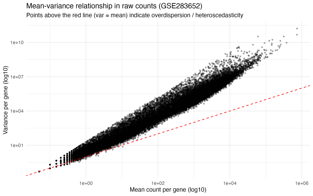
Raw RNA-seq counts are heteroscedastic: genes with higher mean expression also show higher variance. Without filtering and between-sample normalisation, exploratory plots and clustering can be dominated by library-size and compositional artefacts. Even after normalisation, PCA may fail to separate KO from WT if the strongest axes of variation are driven by stromal content or other latent factors rather than genotype.

This project asks: after a disciplined QC and normalisation workflow, do Npy1r KO and WT samples form distinct global expression clusters, and can mouse immune/stromal deconvolution help explain residual structure on the leading principal components?

Our Approach

Data acquisition and metadata alignment

Counts were loaded from the GEO supplementary file and standardised to Ensembl IDs and gene symbols. Phenotype metadata were downloaded with getGEO('GSE283652') and wrangled with dplyr/tidyr to extract genotype and sample identifiers (KO vs WT). Critically, metadata row order was forced to match count-matrix column order with explicit setequal/identical checks, GEO phenoData order is not guaranteed to match supplementary count columns.

Exploratory QC, filtering, and normalisation

The workflow follows a standard edgeR-centred path:

Convert counts to a numeric matrix and visualise mean–SD relationships to document heteroscedasticity in raw PDAC counts.
Build a DGEList, compute log₂-CPM, and inspect sample distributions with violin plots (unfiltered baseline).
Filter lowly expressed genes (keepers with CPM > 1 in at least 10 samples) to remove the zero-inflated bulge that distorts early plots.
Apply TMM (calcNormFactors) to correct compositional bias beyond simple library-size scaling, then re-plot filtered + TMM-normalised log₂-CPM distributions.

Side-by-side violin panels (unfiltered → filtered → TMM) make the effect of each preprocessing step visually auditable.

Mean-variance relationship in RNA-seq counts — Mean–variance structure in count data, the heteroscedasticity that motivates filtering and modelling choices downstream.

Sample structure: clustering and PCA

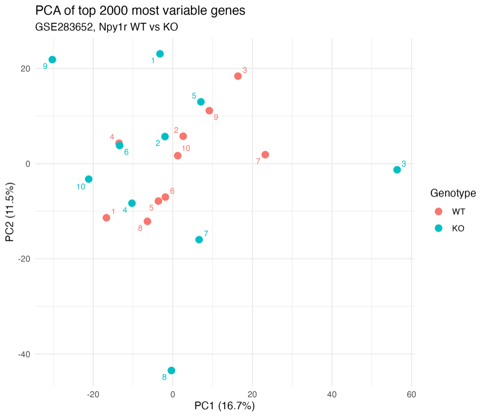
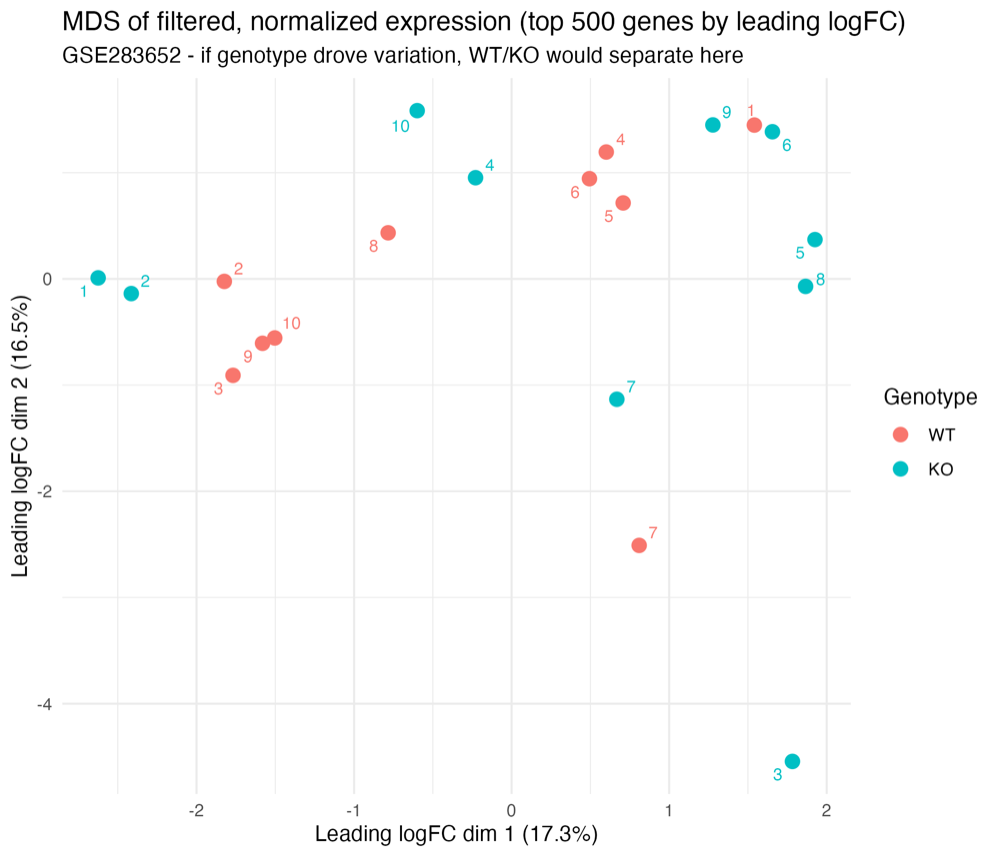
Euclidean distances on transposed filtered, TMM-normalised log₂-CPM were used for hierarchical clustering (Ward.D2 and complete linkage). Principal component analysis (prcomp) summarised global sample structure, with scree plots and PC1–PC2 scatterplots coloured by genotype, plus a “small multiples” view of loadings across PC1–PC8.

PCA of filtered normalised samples — PCA of filtered, normalised samples, used to assess whether genotype drives the dominant axes of variation.

Sample structure MDS plot — Sample-structure view complementary to PCA, highlighting how closely KO and WT libraries sit in expression space.

Deconvolution and PC diagnostics

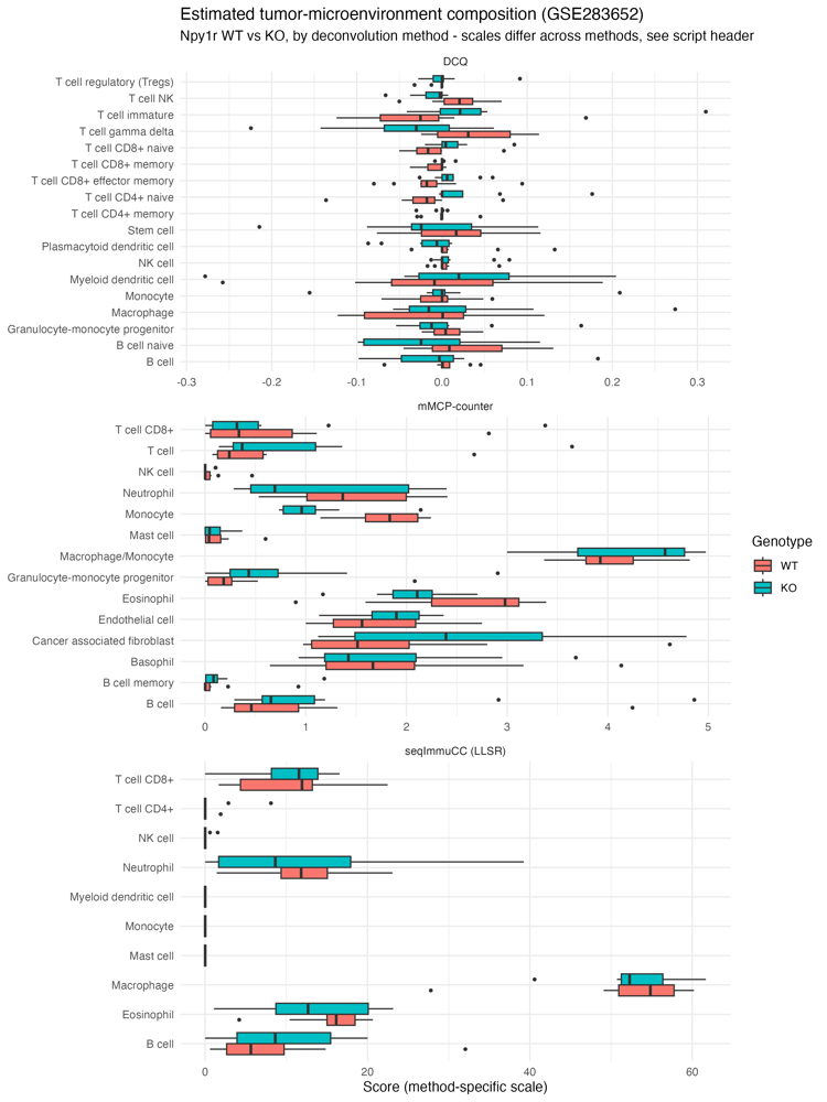
To relate bulk profiles to cell composition, the workflow converts counts toward length-aware abundances (TPM via Ensembl exon lengths from biomaRt for Mus musculus) and explores deconvolution approaches, including EPIC and mouse-oriented immunedeconv / mMCP-counter. Cancer-associated fibroblast (CAF) and other cell-type scores were correlated with PC1 to test whether stromal or immune fractions explain the leading axis of sample variation.

Cell-type deconvolution overview — Deconvolution-style summary of cell-type signals, a bridge between bulk expression structure and tumour microenvironment composition.

Results Overview

Raw counts showed the expected mean–SD fan shape. Filtering removed genes with near-zero expression across samples, and TMM normalisation tightened between-sample log₂-CPM distributions relative to the unfiltered baseline.

On PCA, KO and WT groups did not form cleanly separated clusters: the WT cloud largely sat inside a broader KO ellipse, with substantial overlap. KO replicates also showed greater spread, including samples behaving as relative outliers. PC1 and PC2 together explained a modest fraction of total variance (on the order of ~17.5% and ~12% respectively in the recorded notes), less than 30% combined, indicating that genotype is not a single dominant global effect under these conditions.

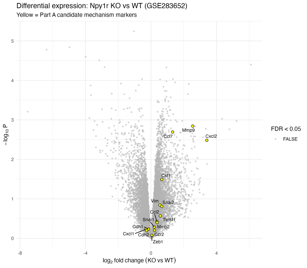
Deconvolution diagnostics were then used to ask whether microenvironment scores track PC1. Correlating cell-type scores (including CAF) with PC coordinates provides a concrete way to decide whether a simple ~ genotype differential expression design is defensible, or whether composition covariates should be considered in follow-up modelling.

Volcano plot Npy1r KO versus WT — Downstream differential expression view (Npy1r KO vs WT), the natural next step once exploratory structure and composition checks are in place.

Conclusion

This project converts a raw GEO PDAC mouse RNA-seq accession into a transparent exploratory narrative: acquire and align metadata carefully, visualise heteroscedasticity, filter and TMM-normalise with edgeR, then interrogate sample structure with clustering and PCA. For GSE283652, the leading global axes do not cleanly separate Npy1r KO from WT, and KO libraries show higher dispersion, a reminder that genotype contrasts in stroma-rich tumours must be interpreted alongside composition and QC.

Mouse-aware deconvolution then links expression space to microenvironment scores, informing whether subsequent differential expression can proceed with a straightforward design matrix or needs composition-aware covariates. The same discipline, check alignment, show each preprocessing step, and explain PCA with biology, scales to other bulk tumour RNA-seq projects.

Source analysis: Pancreatic.R in the pancreatic.cancer.mouse RStudio project (musfira-projects), using GEO accession GSE283652.